Experiment E001 · logbook

Photorealistic 3DGS from our data: how much, where, and why not

From the work order to the evaluation scorecard: real 3D Gaussian Splatting training on the test-gta-demo-1 scene, with the discovery of the navigability envelope and the depth-regularized series. July 1–2, 2026, A10G GPU box.

Question: How much photorealism do we get from a 3DGS trained on our data (gameplay video + poses from the LingBot-MAP reconstruction)? Enough to make it the hero renderer of 3d-viewer?
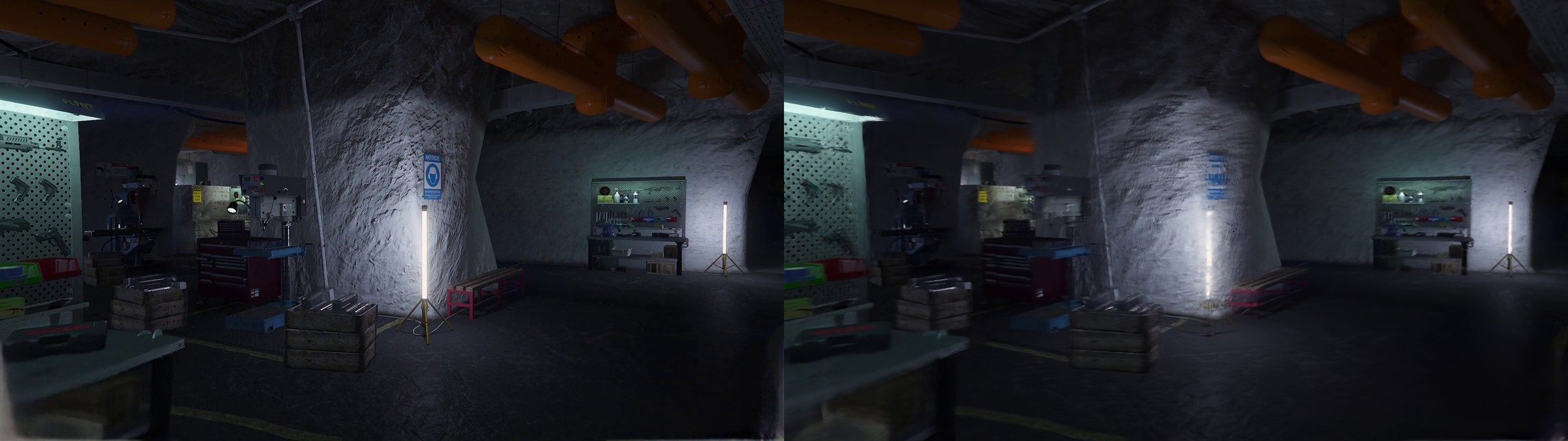
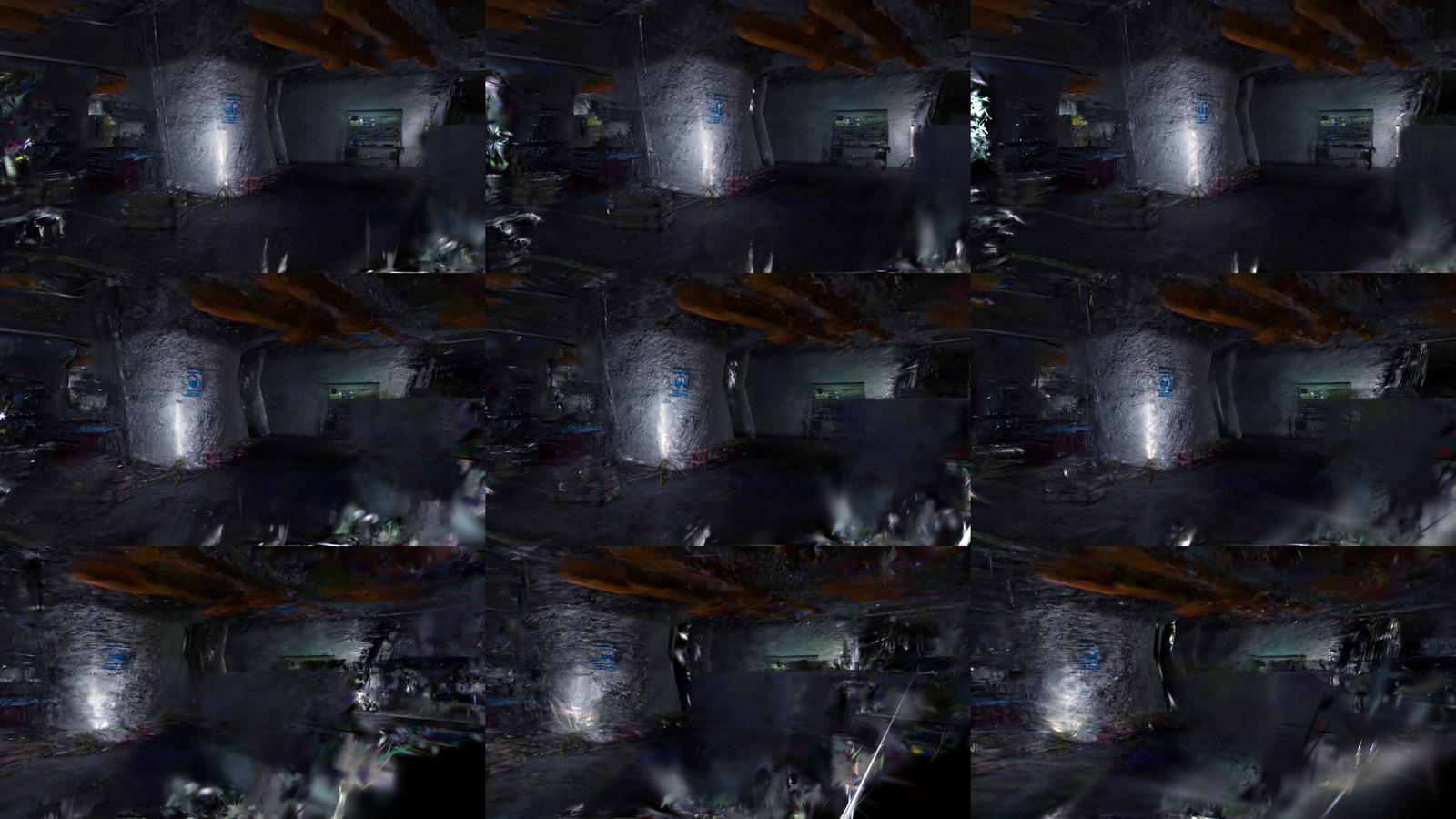
Short answer: Yes along the capture path (PSNR 28.7, solid surfaces, ~90 fps): a clear step up from points. No in free-fly: quality collapses ~20 cm outside the capture corridor (0.9 m), and it is a limit of the capture, not of the optimization — no regularizer moves it.
Where: code and docs: 3d-data-reconstruction/3dgs/ (commit 7a6fbe9) · artifacts: /home/ubuntu/3d-data-reconstruction/testruns/3dgs/test-gta-demo-1/ on the box (453 MB ply, 34 MB spz, 3 checkpoints, COLMAP dataset)
Stack: gsplat 1.5.3 (Apache-2.0) · torch 2.11+cu128 · A10G 24 GB · ~30 min and 4.4 GB VRAM per run

Context

From a video, the 3d-data-reconstruction pipeline (LingBot-MAP, feed-forward) produces per-frame poses, per-pixel depth, and a dense point cloud. 3d-viewer today renders points — the visual ceiling is "colored dots". 3DGS promises real surfaces at the same static-hosting cost. The work order (Marco, Jun 30) asked us to actually train and measure before investing in the integration.

Phase 0 — Tracking down the ingredients · Jul 1

3DGS trains against calibrated images: we needed the 300 source frames and the intrinsics. Neither was where we expected.

The frames: the demo directory does not reference them; the original command, fished out of the bash history, pointed to ProPainter/gta_cave/19-47-44clip_300-600.mp4 (frames 0–299 at 60 fps) — not to the videos in gta_videos/session-2/ that looked like the obvious candidates. The scene is an underground GTA bunker/workshop, not the "shop" from the work order.

The intrinsics: LingBot-MAP predicts them (FOV in the pose encoding) but demo-two.py does not save them. Recovering them became a small result of its own:

Method — pointcloud.npz is exactly depth.npy reprojected through K, confidence-filtered, concatenated in frame/raster order. Frame 0's slice starts at offset 0 by construction: pairing its masked pixels with the cloud's prefix yields exact point↔pixel correspondences up to the first divergence (detected via depth consistency). Least-squares over 63k clean pairs → fx=1100.39, fy=1089.54 @1080p (FOV 82.2°×52.7°), residuals ~1e-5 px, with cx,cy landing on W/2,H/2 exactly as the pipeline code predicts. Script: 3dgs/recover_intrinsics.py.

Abandoned path — reconstructing the correspondence over the entire cloud: it fails because sky-mask regeneration is not bit-stable (~1% of pixels at soft edges change) and the counts never reconcile (43.88M vs 43.40M). Frame 0's clean prefix is enough and provably exact. We also abandoned the idea of re-running the model to get the intrinsics back: pointless GPU cost against a closed-form fit.

Reprojection sanity check (cloud → 4 frames, split-screen overlay): pixel-level alignment across the whole sequence. Only then did we start training.

E1 — Vanilla baseline · Jul 1

gsplat simple_trainer default, 30k iterations, frames at 1600×900, init from 2M cloud points, holdout of 1 frame in 8. Deliberate choice: --no-normalize-world-space, so the gaussians stay in the reconstruction's world frame and everything the viewer already does (fly-through, framing) carries over unchanged.

Abandoned paths — the Inria reference implementation (CC-BY-NC: incompatible with commercial products; gsplat is Apache-2.0 and reproduces the paper); COLMAP from scratch (it lands in an arbitrary coordinate frame and breaks alignment with the cloud and camera path — the LingBot-MAP poses act as free "SfM"); the gsplat master examples (pinned to torch 2.9.1 + NVIDIA dependencies: checkout v1.5.3 aligned with the pip wheel).

step	PSNR	SSIM	LPIPS	gaussians
3k (smoke)	27.14	0.834	0.353	1.76M
30k	28.70	0.852	0.253	1.92M

real frame vs 3DGS render — **Held-out frame 128** — left the real frame (never seen in training), right the render. Emissives, light falloff and readable signs; some high-frequency texture on the rock is lost.

The real discovery — the 300 poses cover a corridor of ~0.9 m. Inside and along the corridor: near-photorealism. 5 cm sideways: edge artifacts. At 10 cm: peripheral smearing. At 20+ cm: splat "spaghetti". Pure rotation from a training pose, on the other hand, holds up. The model has never seen the scene from outside the corridor: it is street-art anamorphosis — perfect from the designated spot, distorted everywhere else. The renderer decision is also a capture-protocol decision.

lateral offset sweep — **Lateral sweep from pose 128** — in reading order: 0 cm, +5, +10, +20 cm. The degradation is gradual but relentless.

E2 — Depth-regularized, and the point cloud exits the stage · Jul 2

Two moves in one. (1) The init no longer reads pointcloud.npz: we reproject depth.npy directly — which is the same thing by construction (verified at float32), so the 3DGS chain sheds a 567 MB artifact. Producer input: frames + poses + depth + K, period. (2) Depth enters the loss: gsplat's --depth_loss supervises disparity on the SfM points anchored to the frames; by sampling 6,700 depth pixels per frame and registering them as COLMAP tracks, the samples become depth anchors without touching the trainer.

run	PSNR	depth err. p50	p90	splats	aniso p99
E1 baseline	28.70	12.45%	32.2%	1.92M	1.6k
E2 depth loss	28.63	4.78%	20.5%	1.88M	2.2k

Lesson — the depth loss fixes the geometry, not the off-path renders. Rendered-depth error drops 2.6× (at identical photometry): great for downstream uses that trust the 3DGS depth (3D labeling, occlusion tests). But the navigation envelope does not move: the anchors live on the same rays as the training frames, and the needle gaussians that cheat along those rays satisfy photometry and depth. The anisotropic tail (p99) stays intact.

E3 — Shape regularizers: half lesson, half own goal · Jul 2

A direct attack on the tail: depth_lambda 5×, scale_reg 0.01 (penalizes large gaussians), opacity_reg 0.001 (discourages floaters).

run	PSNR	depth err. p50	p90	splats	aniso p99
E3 +reg	28.57	3.25%	13.7%	1.43M (−25%)	289k (!)

Instructive own goal — scale_reg penalizes absolute scale: to pay less, the needles got thinner instead of shorter (p99 anisotropy from 1.6k to 289k, bright streaks visible off-path). To be replaced, if anything, with a penalty on the max/min ratio of the scales. opacity_reg, on the other hand, holds up: −25% splats at equal PSNR, faster rendering, smaller file.

off-path comparison baseline / E2 / E3 — **Off-path side by side** (columns: E1 | E2 | E3; rows: +10, +20, +40 cm) — to the eye they are equivalent: confirmation that outside the corridor the bottleneck is the *missing observations*, not the training recipe.

The ablation matrix (read BEFORE launching a run)

Each run costs ~30 min of A10G. Before launching one: check here that the combination has not already been tried, and change one variable at a time. Metrics: PSNR on the 38 held-out frames; depth error = rendered depth vs LingBot depth; aniso = max/min ratio of the scales per gaussian (the p99 tail is the "spaghetti").

run	depth_λ	scale_reg	opacity_reg	PSNR	depth p50	p90	splats	aniso p99	verdict
E1	–	–	–	28.70	12.45%	32.2%	1.92M	1.6k	vanilla baseline
E2	1e-2	–	–	28.63	4.78%	20.5%	1.88M	2.2k	✓ geometry 2.6×, photometry unchanged — clean (single variable)
E3	5e-2	0.01	0.001	28.57	3.25%	13.7%	1.43M	289k	⚠️ 3 variables at once → attribution impossible; scale_reg pathological (thinner needles, not shorter)
E4 — open	5e-2	–	0.001	?					the attribution test: if depth p50 → ~3.3% with healthy aniso, the credit was depth_λ's (and it goes into the producer); if it stays ~4.8%, E3's gain was a scale_reg artifact

Method — E3 is the lesson: three variables in a single run produced the best geometry number and the impossibility of knowing why. From now on: one variable per run, or combinations planned in the table above before launching. Sensible candidates after E4: a penalty on the scale ratio (in place of absolute scale_reg, against the needles), dense depth loss weighted by depth_conf.npy. The producer recipe today is the "E2 + opacity_reg" row — it is updated only with a verified row of this table.

Engineering — the chain is closed · Jul 2

From research result to product, two commands:

# GPU box (3d-data-reconstruction): prep → training (E2+opacity_reg) → scene.sog
python 3dgs/train_gsplat.py --demo-dir <recon> --frames-dir <frames> --intrinsics <K.npz>
# viewer (3d-viewer): bounds + camera path + manifest, no GPU
python build_scene.py <recon> --name <scene> --producer gsplat --gsplat-asset <scene.sog>

The split respects the repo separation: training (GPU, conda) lives with the pipeline; 3d-viewer receives only the ready-made .sog and stays display+navigation. Rendering in the viewer is Spark 2.1 on modern three.js, isolated from Potree's ancient three; camera path and fly-through unchanged. End-to-end smoke test at 300 steps: it already paid for itself by catching a relative-path bug before the first real run.

Where we are, what remains open

Producer config: E2 recipe (init from depth + depth loss) + opacity_reg, no scale_reg — it changes only with a verified row of the ablation matrix.

Confidence-weighted dense depth loss — today we use 6.7k anchors/frame out of 1.44M pixels and depth_conf.npy only as a binary filter; a dense L1 on the render's depth channel is a small patch to the trainer.
Capture protocol — the structural answer to free-fly: wide-baseline passes over the same scene. To be tried as soon as the capture pipeline allows it.
Browser verification — ✅ done (Jul 2): loadGsplat() implemented in 3d-viewer with Spark 2.1 + modern three.js (engine separate from Potree's ancient three, same Z-up space: camera path and fly-through unchanged). Format surprise: splat-transform 2.7's .spz is version 4, which Spark rejects — solved by exporting .sog (27 MB, even smaller). The 1.92M-splat scene renders from the first pose with the trajectory overlaid (verified headless with SwiftShader). The gsplat producer is closed as well — see "Engineering" above.
Product direction — 3D spatial labeling while navigating the scene: 3DGS as the display layer, labels computed in the shared world frame (which we preserved on purpose), grounding on posed RGB-D.

Logbook convention: one page per experiment campaign, in chronological order; decisions in the terracotta callouts, abandoned paths (with reasoning) in the gray callouts, surprises in olive green. Numbers always in a table; heavy artifacts stay on the box with the path noted in the scorecard.